Probability and Statistics: Assignment 4

Modify the code below so that it plots \(y=x^3\) over the interval \([-1,3]\).
```
x = seq(-2, 2, by = 0.1)
y = x^2
plot(x, y, col = "skyblue", type="l")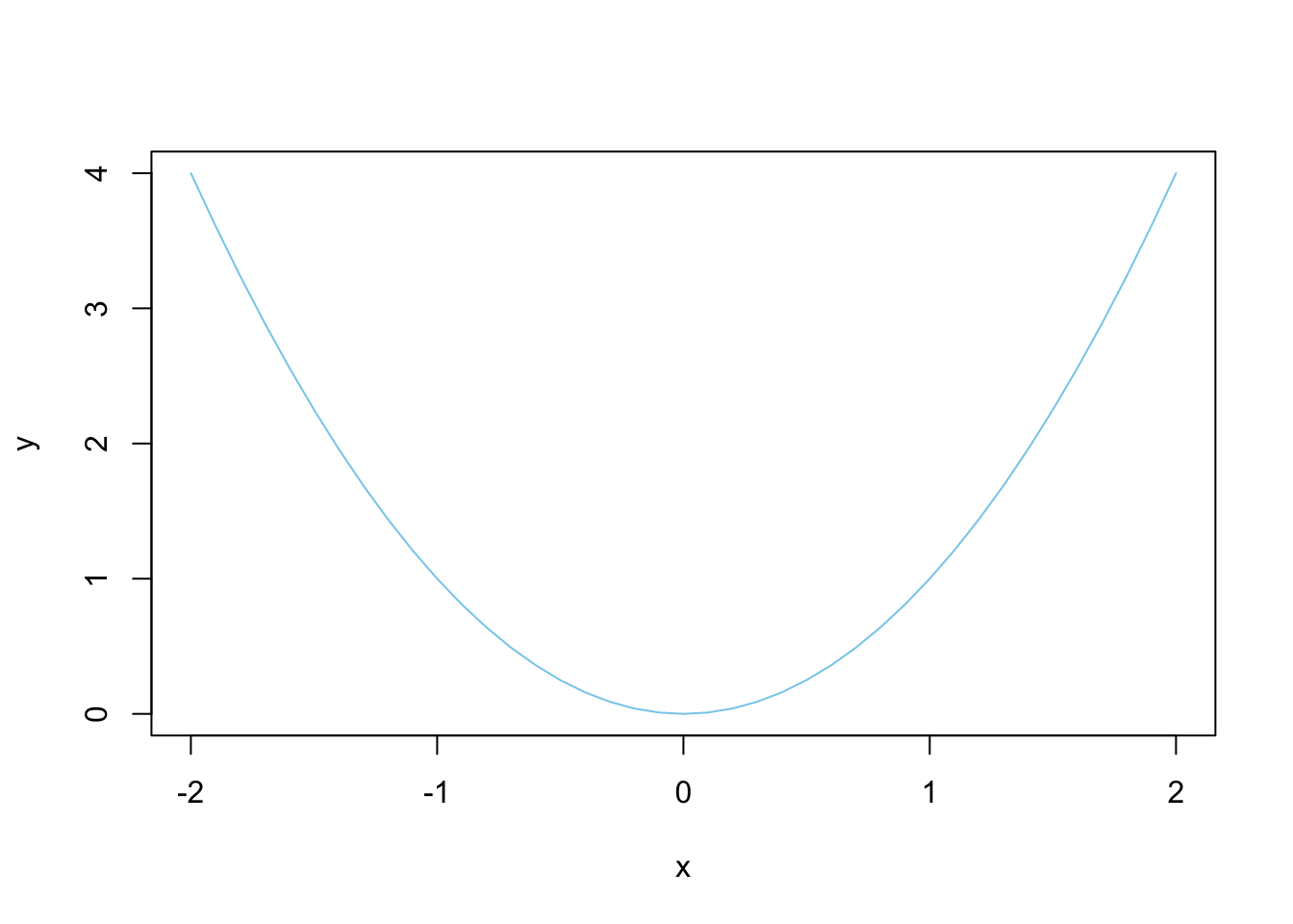
```
Exercise 4.3
Use simulation to estimate the probabilities you found in the previous problem.
```
# Use this code chunk.
```
Consider the random variable that “picks” a number between 0 and 1 with the pdf given by

\[f(x) = \begin{cases} 6x(1-x), & x\in[0,1] \\ 0 & \text{otherwise}\end{cases}.\]
1. Plot this density function.
```
# Use this code chunk.
```
1. Write code to estimate the integral.
```
# Use this code chunk.
```
1. Calculate the exact integral to show that \(f(x)\) is, indeed, a probability density function.
Let \(X\) be a normal rv with mean 0 and standard deviation 1.
1. Plot the density function.
```
# Use this code chunk.
```
1. Write code to estimate the integral.
```
# Use this code chunk.
```
1. How much of the density is no more than 2 standard deviations away from the mean?
```
# Use this code chunk.
```
1. How much of the density is no more than 1 standard deviation away from the mean?
```
# Use this code chunk.
```
1. Exercise 4.5.b. Also provide a plot.
```
# Use this code chunk.
```