Approximating a distribution by a large sample
I will illustrate this with a beta distribution. Here’s a plot of the pdf for \(X\sim Beta(15,7)\):
beta_pdf <- tibble(
  theta = seq(0, 1, by = 0.01),
  p_theta = dbeta(theta, 15, 7)
)
beta_pdf %>%
  ggplot(aes(theta, p_theta)) +
  geom_line()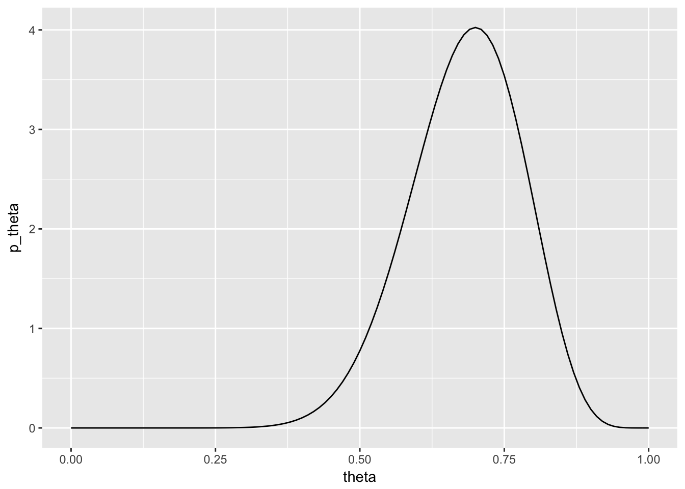
I can also generate lots of data drawn from this distribution and then produce a (relative frequency) histogram for the data:
beta_data <- tibble(
  theta = rbeta(50000, 15, 7)
)
beta_data %>%
  ggplot(aes(theta)) +
  geom_histogram(aes(y = ..density..), binwidth = 0.02)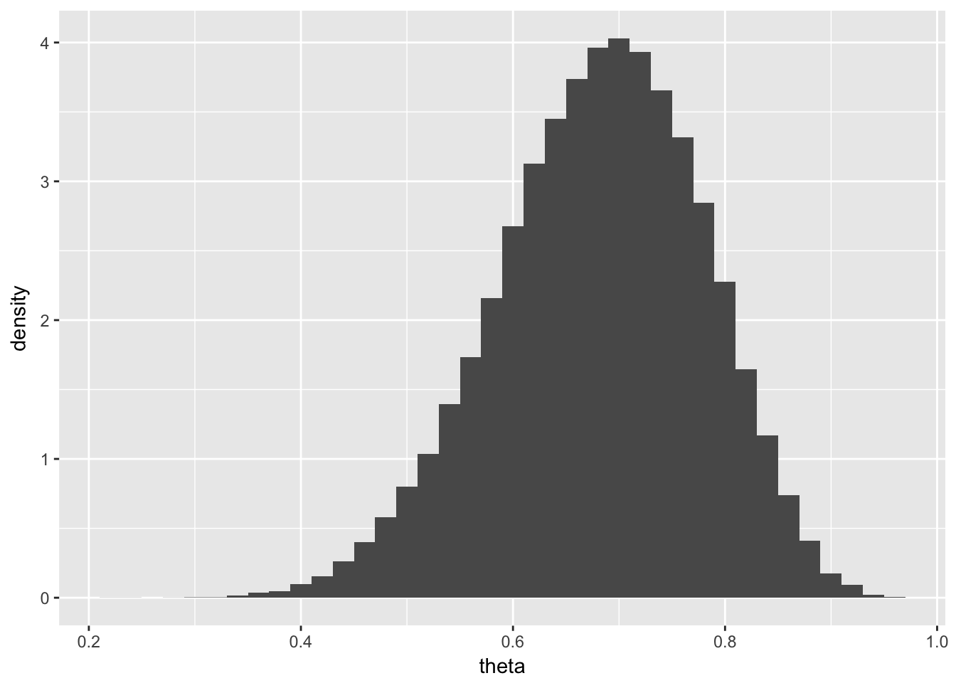
If I have a sufficient amount of data, then the density plot should have the same shape as the pdf:
ggplot(beta_pdf, aes(x = theta)) +
  geom_line(aes(y = p_theta), col = "blue") +
  geom_histogram(data = beta_data, aes(y = ..density..), binwidth = 0.02)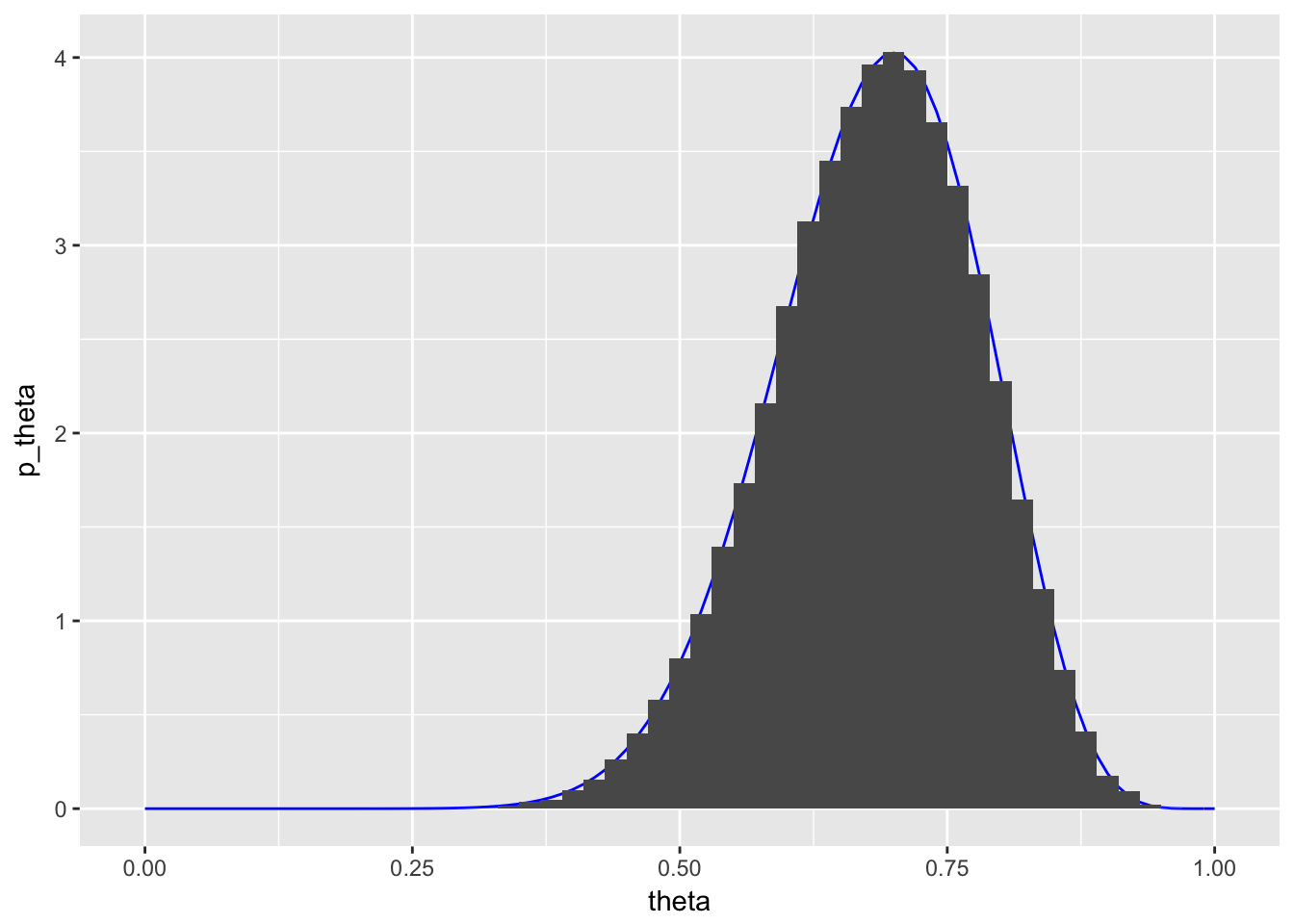
I was able to generate this data very easily since I know the distribution it comes from. The simple command, rbeta(50000, 15, 7), gives me 50000 random values from \(Beta(15,7)\).
We’re looking for a way, however, to generate such data without knowledge of the distribution.
Simple Case of Metropolis Algorithm
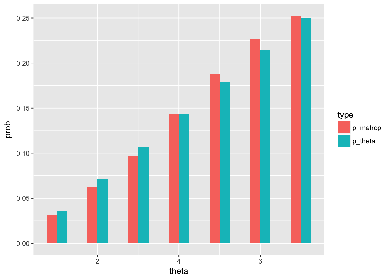
Consider the simple example outlined in section 7.2 of the book where \(\Theta\) is a discrete random variable with \(p(\theta)=0\) for \(\theta\not\in\{1,2,...,7\}\). Suppose that data D has been collected and that the “numerator function” (see text and class notes) is given by:
\[p(D|\theta)p(\theta)=\theta\]
The target distribution is proportional to this function. Why? In the homework you were asked to write a function that would generate a random sample from the target distribution using the Metropolis algorithm.
Your results should that show the distribution of the random sample produced via the Metropolis algorithm is nearly the same as the distribution of the (in this case, known) posterior:
Metropolis algorithm more generally
Estimating Bias in One Coin
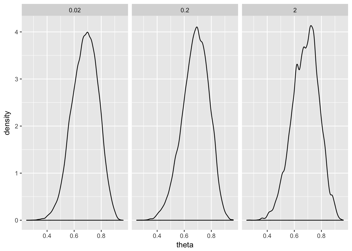
We first apply the metropolis algorithm to infer the bias of a single coin. Assume an uninformative prior; let \(\Theta\sim Beta(1,1)\). Now we flip the coin 20 times and get 14 heads. Now we will sample the posterior via the Metropolis algorithm, using a normal proposal distribution with mean 0 and standard deviation values of 0.02, 0.2, and 2. These samples provide an estimate of the posterior distribution:
Estimating Bias in Two Coins
We now want to infer the bias of two coins. First, we will look at this problem analytically. Then, we will apply the metropolis algorithm to solve the same problem.
Solving the problem analytically
Let \(\Theta_1\) and \(\Theta_2\) be independent beta priors with \(\Theta_1\sim Beta(2,2)\) and \(\Theta_2\sim Beta(2,2)\). Now we flip the first coin 8 times and get 6 heads and we flip the second coin 7 times and get 2 heads.
In the homework, you will show that with independent Beta priors and Bernoulli likelihoods, the posterior consists also of independent Beta distributions. Since we know these things analytically, it’s a good opportunity to visualize these distributions.
z_1 <- 6
N_1 <- 8
z_2 <- 2
N_2 <- 7
coins_df <- tibble(
  theta_1 = seq(0, 1, by = 0.01),
  theta_2 = seq(0, 1, by = 0.01)
) %>%
  data_grid(theta_1, theta_2) %>%
  mutate(
    prior = dbeta(theta_1, 2, 2) * dbeta(theta_2, 2, 2),
    prior = prior / sum(prior),
    likelihood = (theta_1 ^ z_1 * (1 - theta_1) ^ (N_1 - z_1)) *
      (theta_2 ^ z_2 * (1 - theta_2) ^ (N_2 - z_2)),
    likelihood = likelihood / sum(likelihood),
    posterior = dbeta(theta_1, 2 + z_1, 2 + N_1 - z_1) *
      dbeta(theta_2, 2 + z_2, 2 + N_2 - z_2),
    posterior = posterior / sum(posterior)
  )
Here’s a 3-D surface plot of the prior and the corresponding contour plot below it:
# plotly mesh plots
coins_df %>%
  plot_ly(x = ~theta_1, y = ~theta_2, z = ~prior, type = 'mesh3d')
coins_df %>%
ggplot(aes(theta_1, theta_2, z = prior)) + geom_contour()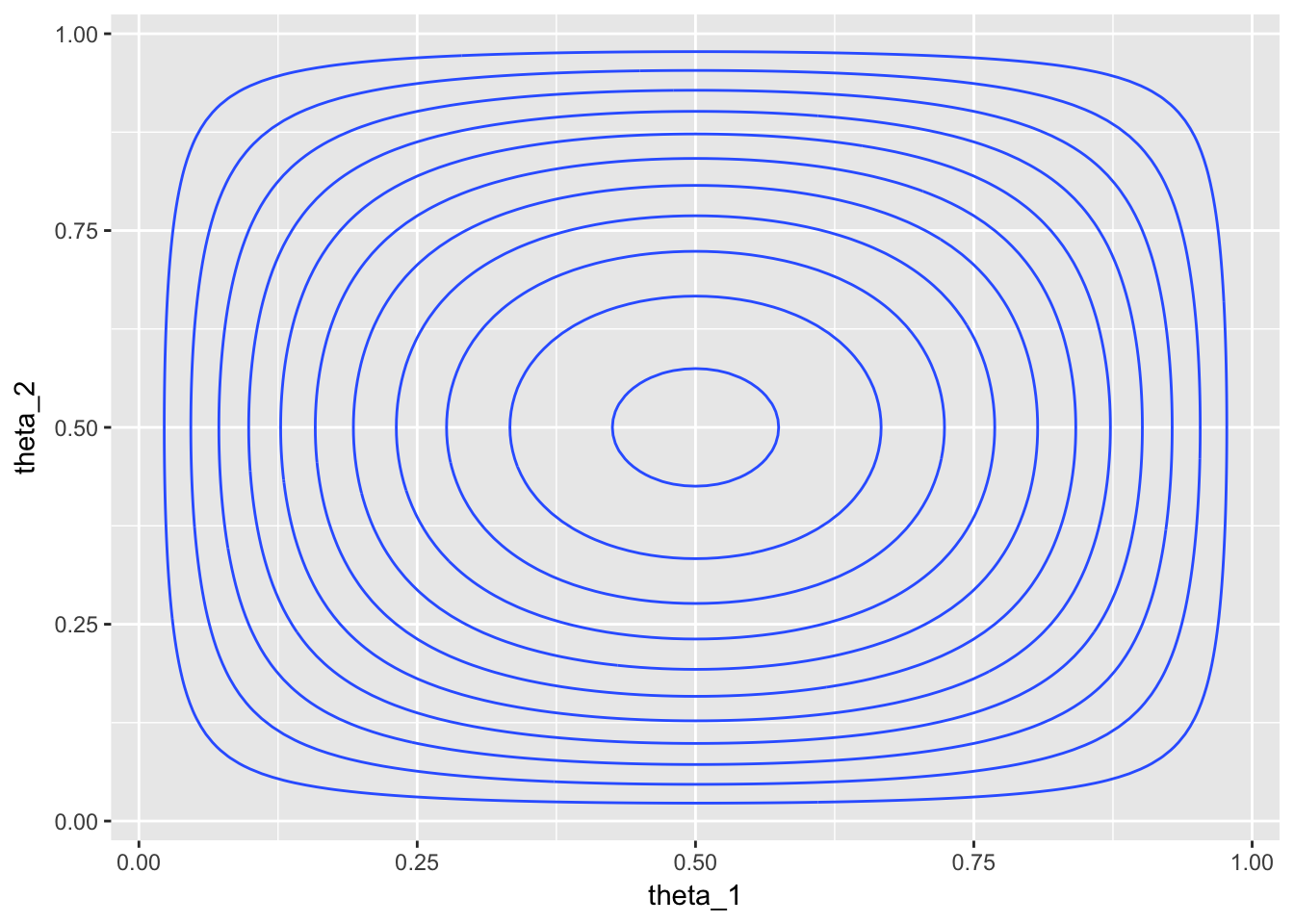
Here’s a 3-D surface plot of the likelihood and the corresponding contour plot below it:
coins_df %>%
  plot_ly(x = ~theta_1, y = ~theta_2, z = ~likelihood, type = 'mesh3d')
coins_df %>%
ggplot(aes(theta_1, theta_2, z = likelihood)) +
geom_contour() +
xlim(0, 1) + ylim(0, 1)
Here’s a 3-D surface plot of the posterior and the corresponding contour plot below it:
coins_df %>%
  plot_ly(x = ~theta_1, y = ~theta_2, z = ~posterior, type = 'mesh3d')
coins_df %>%
ggplot(aes(theta_1, theta_2, z = posterior)) +
geom_contour() +
xlim(0, 1) + ylim(0, 1)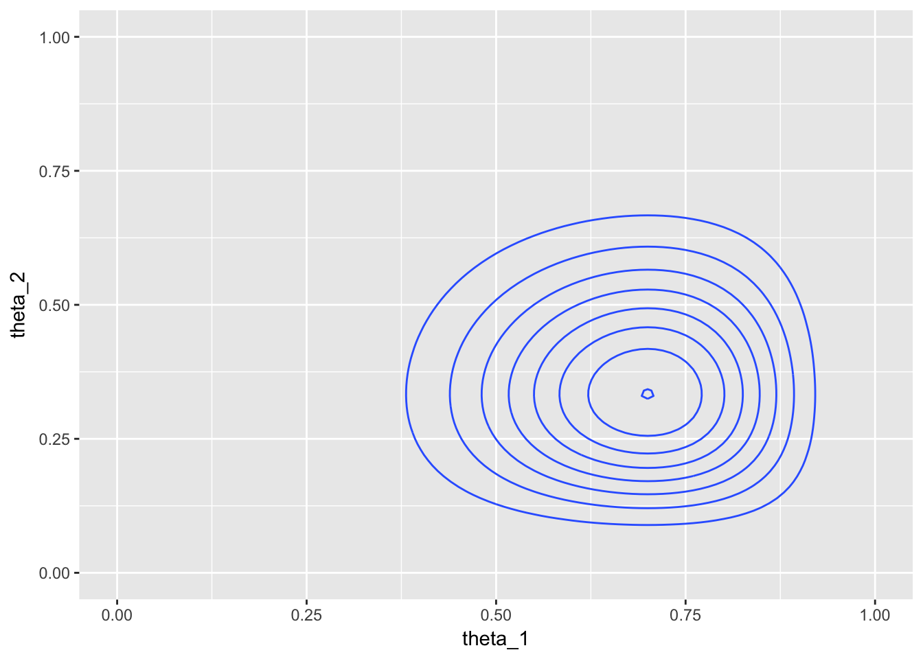
All three contour plots:
coins_df %>%
  gather(type, prob, -theta_1, -theta_2) %>%
  mutate(type = factor(type, levels = c("prior", "likelihood", "posterior"))) %>%
  ggplot(aes(theta_1, theta_2, z = prob)) +
    geom_contour(col = "cornflowerblue") +
    facet_wrap(~type, ncol = 1, scales = "fixed")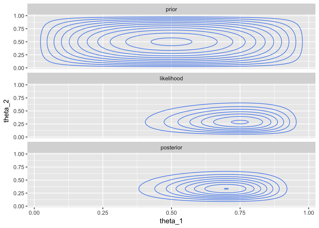
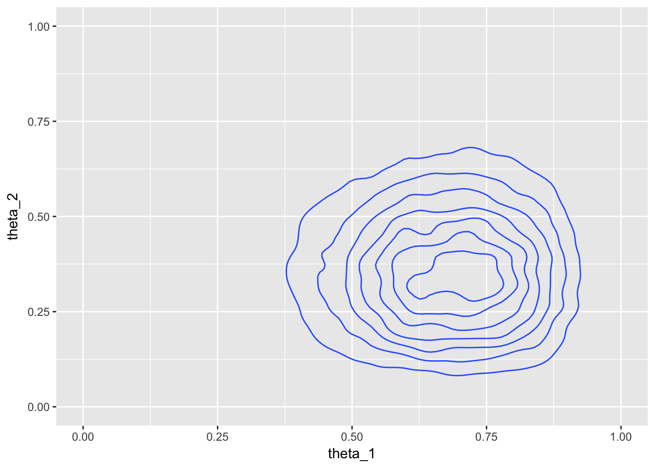
Solving the problem via the Metropolis algorithm
In the homework, you are asked to solve the same problem via the Metropolis algorithm.
metrop_df <- metropolis(thetas, numerator_bern_beta, data, prop_sd = 0.02)

metrop_df %>%
  ggplot(aes(theta_1, theta_2)) +
    geom_density_2d() +
    xlim(0, 1) + ylim(0, 1)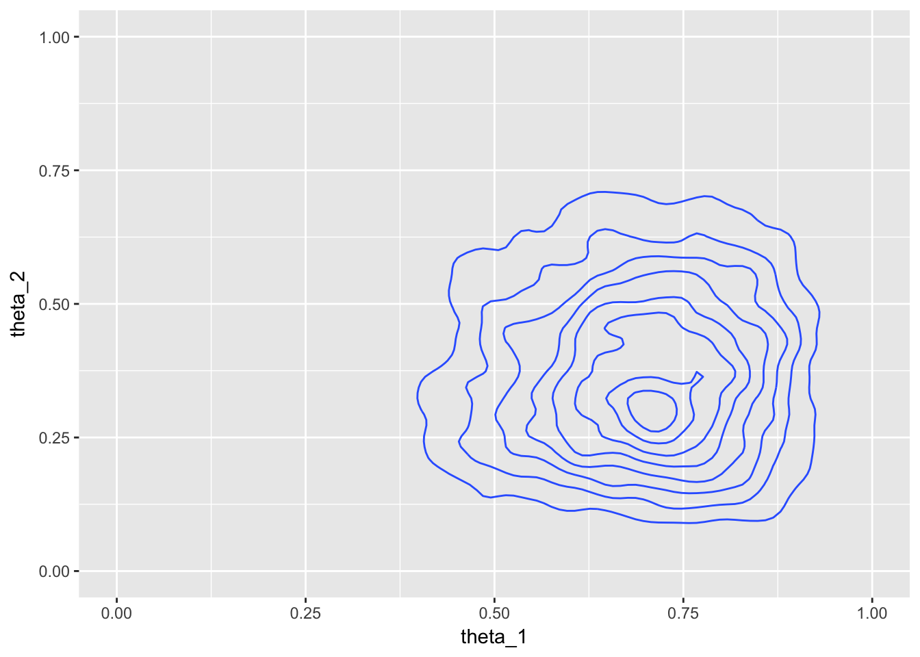
metrop_df <- metropolis(thetas, numerator_bern_beta, data, prop_sd = 0.2)

metrop_df %>%
  ggplot(aes(theta_1, theta_2)) +
    geom_density_2d() +
    xlim(0, 1) + ylim(0, 1)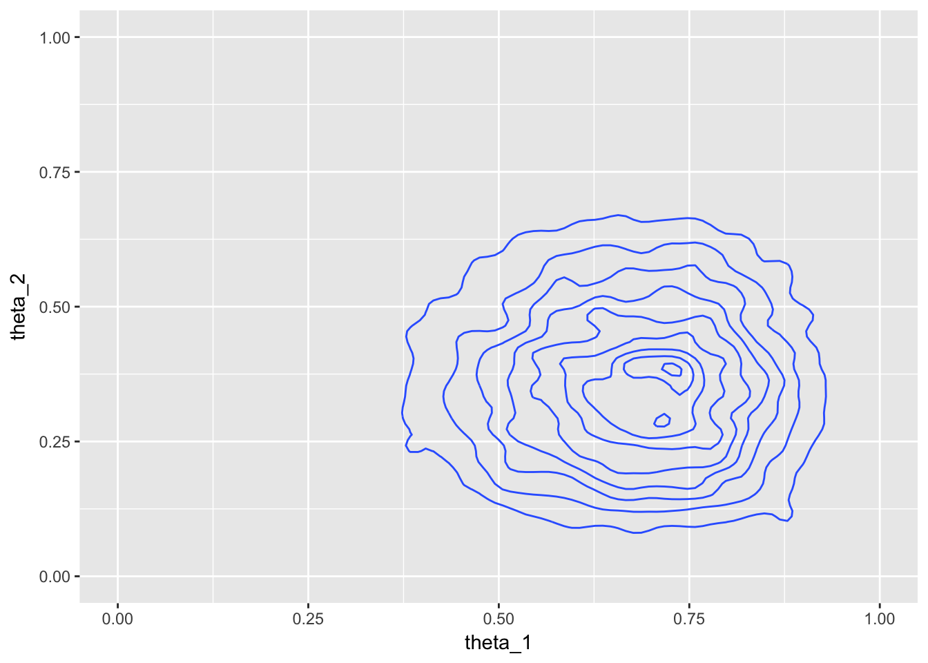
Gibbs sampling
The Metropolis algorithm can be inefficient. Under certain conditions there may be alternative methods available that are more efficient. Gibbs sampling is one such method.
Here is an implementation of Gibbs sampling to solve the two coin problem:
gibbs <- function(parms, f, D, N = 25000) { # parms is a list; D is a list
  l <- parms
  n <- length(l)
  p <- matrix(0, N, n, dimnames = list(NULL, names(l)))
  for (i in 1:n) {
    p[1,i] <- runif(1, min = min(l[[i]]), max = max(l[[i]]))
  }
  idx <- 1
  for (i in 2:N) {
    p[i, ] <- p[i - 1, ]
    p[i, idx] <- f(D[[idx]])
    idx <- idx %% n + 1
  }
  as_tibble(p)
}

cond_post <- function(D) { # prior is beta(2,2)
  shp1 <- 2 + D[[2]]
  shp2 <- 2 + D[[1]] - D[[2]]
  rbeta(1, shp1, shp2)
}

thetas <- list(
  theta_1 = c(0,1),
  theta_2 = c(0,1)
)

data <- list(
   D_1 <- list(N_1 = 8, z_1 = 6),
   D_2 <- list(N_2 = 7, z_2 = 2)
 )

gibbs_df <- gibbs(thetas, cond_post, data)

gibbs_df %>%
  ggplot(aes(theta_1, theta_2)) +
    geom_density_2d() +
    xlim(0, 1) + ylim(0, 1)