Background
Sample Spaces and Events
An experiment is any action or process whose outcome is subject to uncertainty. The sample space of an experiment, denoted \(\mathcal S\), is the set of all possible outcomes of that experiment. An event is any subset of \(\mathcal S\).
Axioms of Probability
Let \(\mathcal{S}\) be a sample space, \(E\) an event and \(\{E_1, E_2, ... \}\) a countable collection of pairwise disjoint events. Then,
- \(P(E)\geq 0\)
- \(P(\mathcal{S})=1\)
- \(P\left(\bigcup\limits_{i=1}^{\infty} E_{i}\right) = \sum\limits_{i=1}^{\infty} P(E_i)\)
Random Variable
Let \(\mathcal{S}\) be a sample space and let \(X:\mathcal{S}\rightarrow\mathbb{R}\). Then \(X\) is a random variable.
Example: For a coin toss we have \(\mathcal{S}=\{T, H\}\). Let \(X:\mathcal{S}\rightarrow\mathbb{R}\) with \(X(T)=0\) and \(X(H)=1\).
A random variable is a discrete random variable if its set of values is countable. A random variable is continuous if its set of values is an interval. (That’s not quite accurate, but it’s good enough.)
Probability Distributions
When probabilities are assigned to the outcomes in \(\mathcal{S}\), these in turn determine probabilities associated with the values of any random variable \(X\) defined on \(\mathcal{S}\). The probability distribution of \(X\) describes how the total probability of 1 is distributed among the values of \(X\).
Probability Mass Function (pmf)
Let \(X:\mathcal{S}\rightarrow\mathbb{R}\) be a discrete random variable. The probability mass function of \(X\) (pmf) is the function \(p:\mathbb{R}\rightarrow[0,1]\) such that for all \(x\in\mathbb{R}\), \(p(x)=P(X=x)\).
Example: The pmf for the random variable in the previous example where the probability of heads is \(\theta\) is given by
\[p(x) = \begin{cases} 1-\theta & \text{if } x=0 \\ \theta & \text{if } x=1 \\ 0 & \text{otherwise} \end{cases} \]
Probability mass functions can be visualized with a line graph. For \(\theta = 0.2, 0.5,\) and \(0.8\):

It’s worth noting a couple of properties of a pmf:
- \(p(x)\geq 0, x \in \mathbb R\)
- \(p(x)=0, x \notin X(\mathcal S)\)
- \(\sum_{x\in X(\mathcal S)}p(x)=1\)
Before moving on to continuous rv’s, a couple more examples.
Example: Consider the experiment of tossing a coin twice and counting the number of heads. Give the sample space, define a sensible random variable and draw a line graph for the pmf.
Solution: \(\mathcal{S}=\{TT, TH, HT, HH\}\). Define \(X:\mathcal{S}\rightarrow\mathbb{R}\) by \(X(TT)=0\), \(X(TH)=X(HT)=1\) and \(X(HH)=2\). Then the pmf is given by
\[p(x) = \begin{cases} 0.25 & \text{if } x=0 \\ .5 & \text{if } x=1 \\ 0.25 & \text{if } x=2 \\ 0 & \text{otherwise} \end{cases} \]
ex1_df <- tibble(
  x = c(0,1,2),
  p_x = c(0.25, 0.5, 0.25)
)
ex1_df %>% ggplot(aes(x, p_x)) +
  geom_col(width = 0.01) +
  geom_point()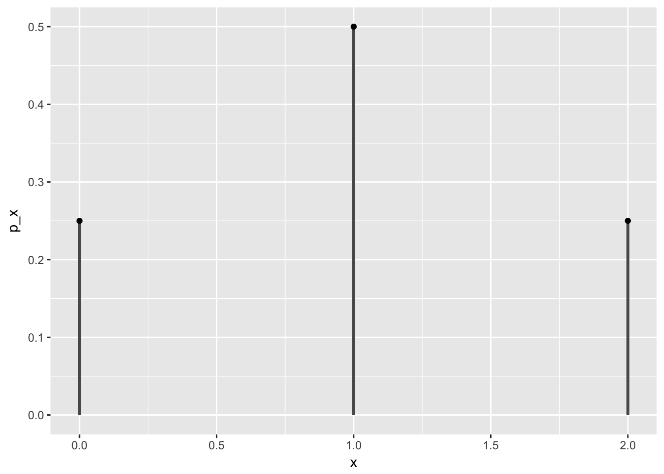
Example: Consider the experiment of tossing a biased coin (where the probability of heads is \(\theta\)) until it lands on heads. Give the sample space, define a sensible random variable and draw a line graph for the pmf.
Solution: \(\mathcal{S}=\{H, TH, TTH, TTTH, ...\}\). Define \(X:\mathcal{S}\rightarrow\mathbb{R}\) by the number of flips required. Then the pmf is given by
\[p(x) = \begin{cases} (1-\theta)^{x-1}\theta, & x=1,2,3,... \\ 0 & \text{otherwise} \end{cases} \]
Probability Density Function (pdf)
Let \(X\) be a continuous random variable. The probability density function of \(X\) (pdf) is a function \(f(x)\) such that for \(a\leq b\),
\[P(a\leq X\leq b)=\int_a^b f(x)\,dx.\]
A couple of properties:
- \(f(x)\geq 0, x\in\mathbb R\)
- \(\int_{-\infty}^{\infty}f(x)\,dx=1\)
- \(P(X=c)=\int_c^c f(x)\,dx=0\)
Example: A uniform random variable on \([a,b]\) is a model for “pick a random number between a and b.” The pdf is given by
\[f(x) = \begin{cases} \frac{1}{b-a}, & x\in[a,b] \\ 0 & \text{otherwise} \end{cases}. \]
Example: Let \(X\) be normal random variable. Then \(X\) has the pdf given by
\[f(x) = \frac{1}{\sqrt{2\pi\sigma^2}}e^{-\frac{(x-\mu)^2}{2\sigma^2}}\]
where \(\mu\) and \(\sigma^2\) are the mean and variance of \(X\). These are properties of \(X\) that we now discuss.
Mean and Variance
Let \(X\) be a random variable. The mean or expected value of \(X\) is defined by
\[\mathbb E(X)= \begin{cases} \displaystyle\sum_{x\in X(\mathcal S)}x\cdot p(x), & X \text{ discrete} \\ \displaystyle\int_{-\infty}^{\infty}x\cdot f(x)\, dx, & X \text{ continuous} \end{cases} .\]
The variance of \(X\) is given by
\[\mathbb V(X)=\mathbb E\left((X - \mathbb E(X))^2\right).\]
The expected value is often denoted \(\mu\) and the variance, \(\sigma^2\). The square root of the variance, \(\sigma\), is called the standard deviation.
Highest density interval
The mean gives us one way to quantify the central tendency of a distribution. Variance is one way to quantify the spread of a distribution. Another way to quantify the spread of a distribution is to specify the highest density interval (HDI). The 95% HDI for a distribution, for example, is an interval \(I\) such that for \(x\in I\), \(f(x)>W\) for some fixed \(W\) and
\[\int_I f(x)\,dx = 0.95.\]
Using R to plot a normal random variable.
We include some code here for plotting the pdf shown on page 83 in the text. This is the pdf of a normal rv with mean 0 and standard deviation 0.2.
f <- function(x) (1 / sqrt(2 * pi * sig ^ 2)) * exp(-(x - mu) ^ 2 / 2 / sig ^ 2)
dx <- 0.01
x <- seq(-0.6, 0.6, by = dx)
mu <- 0
sig <- 0.2
plot(x, f(x), type = "l")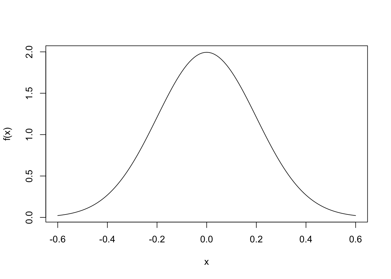
We can estimate the area under this curve. What should it be close to? Why?
sum(f(x)[-1]*dx)## [1] 0.9972947How much of the density is between \(x=-0.2\) and \(0.2\)?
sum(f(seq(-0.2, 0.2, by = dx))[-1]*dx)## [1] 0.6825887